Portfolio Theory for DeFi: Why Systematic Allocation Beats Token Picking

In our previous article, we explored the fundamentals of risk in DeFi, explaining how volatility, geometric returns, and time horizons impact investment outcomes. A key insight emerged: understanding statistical properties of crypto assets is essential for making informed decisions about vault selection.

Now, we're taking the next step: applying rigorous portfolio theory to DeFi investing. While most crypto users chase the next hot token, hoping for life-changing gains, data consistently shows that systematic portfolio allocation delivers superior risk-adjusted returns over time.

The Evolution of DeFi Investing

Before diving into portfolio construction, it's worth considering how DeFi investing has evolved:

2020-2021 ("DeFi Summer"): Characterized by speculative yield farming, governance token airdrops, and triple-digit APYs that inevitably collapsed 2022-2023 (Bear Market): Focus shifted to sustainable yield from lending, staking, and established protocols as many speculative projects failed 2024-2025 (Maturity): Institutional adoption, improved risk management, and the rise of systematic approaches to DeFi investing.

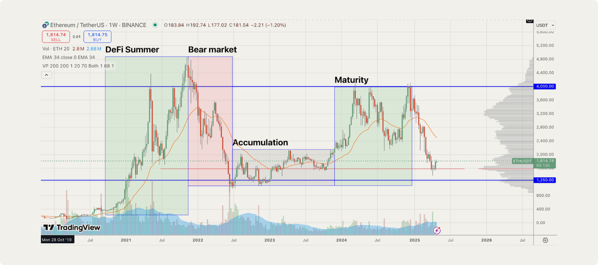
This evolution mirrors traditional finance's development, where early speculation gradually gave way to more sophisticated portfolio approaches. Today's DeFi landscape, with improved infrastructure and liquidity, enables truly systematic investing that was previously impractical.

The Asset Model: Beyond Simple Categorization

At Levva, we've developed a framework that classifies DeFi investments into primary categories:

1. Volatile Assets: Primarily ETH and BTC exposure (via liquid restaking tokens)
2. Safe Yield: Lending protocols and yield-bearing stablecoins

While we operationally use this two-asset model for its simplicity and efficiency, we recognize the nuanced reality of crypto correlations.

Correlation Analysis: When Simplified Models Meet Complex Reality

The correlation between crypto assets isn't static and can vary significantly across different market regimes. Based on our analysis of 60-day rolling correlations from January 2023 to April 2025:

This data reveals important insights:

• BTC-ETH correlation has declined from historical averages of ~0.8 to around 0.7
• During certain periods (notably early 2024), correlations dropped dramatically to as low as 0.2-0.3
• Market regime significantly impacts correlation patterns, with generally higher correlations during uptrends
• Even ERC-20 tokens like LDO, AAVE, and MKR show substantial correlation variability despite their close ecosystem ties to ETH

Notably, during specific narrative-driven cycles (like the L2 expansion in late 2023), correlations can temporarily break down, creating potential diversification opportunities.

Why We Maintain the Two-Asset Framework

Despite the correlation variability shown above, our two-asset framework remains our operational approach for several reasons:

1. Practical Implementation: While correlations do vary, they remain positive and substantial enough (averaging 0.65-0.70) that the implementation benefits of a simplified model outweigh the marginal diversification gains from more complex categorization.
2. Regime Adaptability: Our portfolio construction incorporates the reality of changing correlations through:
   • Regular rebalancing that implicitly adjusts to correlation shifts
   • Timing strategies that can respond to changing market conditions
   • Concentration limits that prevent overexposure during correlation breakdowns
3. Statistical Significance: Even with periods of lower correlation, the sample size required to statistically validate the superiority of more complex models exceeds our available data, essentially facing the same statistical challenge we highlighted with yield sources.
4. Cost-Benefit Analysis: For most users, the gas costs, operational complexity, and monitoring requirements of a more granular asset model would exceed the expected benefits from capturing temporary decorrelation periods.

That said, our vaults capture some of these decorrelation benefits naturally. During periods when certain altcoins become less correlated with ETH, their price movements create rebalancing opportunities that our threshold-based approach automatically captures.

Three Optimization Strategies for Different Risk Profiles

Using our asset framework, we construct three distinct portfolios optimized for different investor objectives:

1. Maximum Sharpe Ratio Portfolio (Ultra Safe)

Optimization Problem: Maximize the ratio of excess return to volatility

Max SR = (Rp - Rf) / σp

Where:

• Rp = Portfolio return
• Rf = Risk-free rate
• σp = Portfolio volatility

Solution: In our model, the Maximum Sharpe Ratio portfolio allocates 100% to Safe Yield and 0% to Volatile Assets.

Why? The incremental return offered by volatile assets doesn't compensate for their dramatically higher volatility. For risk-averse investors prioritizing consistent, risk-adjusted returns, this portfolio maximizes efficiency.

Ideal For: The "Ultra Safe" investor category—individuals or institutions new to DeFi who want simplified "one-click" exposure to DeFi yields while minimizing volatility.

2. Risk Parity Portfolio (Safe)

Optimization Problem: Equalize the risk contribution from each asset class

Risk Contribution(i) = wi × (σi × ρi,p / σp)

Where:

• wi = Weight of asset i
• σi = Volatility of asset i
• ρi,p = Correlation of asset i with the portfolio
• σp = Portfolio volatility

Solution: In our model, the Risk Parity portfolio allocates 93.75% to Safe Yield and 6.25% to Volatile Assets.

Why? Risk parity accounts for the massive volatility difference between crypto and yield-bearing assets, creating equal risk contribution despite the uneven allocation. This provides modest exposure to crypto upside while maintaining relatively stable portfolio behavior.

Ideal For: The "Safe" investor category—users familiar with DeFi who understand the risks but want a balanced approach with controlled exposure to volatile assets.

3. Maximum Geometric Mean Portfolio (Brave)

Optimization Problem: Maximize the expected long-term growth rate

Max GM = arithmetic mean - (variance / 2)

Where:

• Arithmetic mean = Weighted average of expected returns
• Variance = Overall portfolio variance

Solution: In our model, the Maximum Geometric Mean portfolio allocates 72.5% to Safe Yield and 27.5% to Volatile Assets.

Why? This portfolio maximizes expected long-term growth, taking on more short-term volatility in pursuit of higher returns. It recognizes the power of geometric compounding while still maintaining significant risk control compared to pure crypto exposure.

Ideal For: The "Brave" investor category—advanced crypto and DeFi users with longer time horizons who can tolerate moderate volatility for enhanced returns.

Portfolio Comparison: Return, Risk, and Efficiency

Based on our updated correlation data and analysis, let's compare these portfolios quantitatively:

Note: These allocations reflect the updated correlation data showing lower correlation between Safe Yield and Volatile Assets (0.2 average vs. our previous 0.3 assumption).

Data and Methodology Transparency

The figures above are based on:

• Historical data from January 2021 to March 2025
• 60-day rolling correlations calculated across different market regimes
• Volatility measures derived from daily returns
• Forward-looking estimates adjusted for current market conditions (reducing historical ETH returns from ~30% to a more conservative 15%)

It's important to acknowledge that these are estimates subject to uncertainty. To address this, we routinely perform a sensitivity analysis to test how our allocations would change under different scenarios:

This sensitivity analysis helps prevent over-optimization and ensures our allocations remain robust across different market conditions. Note that the Risk Parity and Maximum GM allocations have been adjusted (compared to what we’ve stated elsewhere) to reflect our updated correlation data.

When we apply these allocations to historical market regimes (as defined in our correlation analysis), we observe the following performance characteristics:

The Volatility Tax in Action

The results above demonstrate a counter-intuitive finding: the 100% ETH portfolio has a lower expected geometric return than even the conservative Maximum SR portfolio, despite ETH's much higher arithmetic mean return. This vividly illustrates the "volatility tax" concept.

Consider this simplified example:

Imagine investing $10,000 in ETH with 60% annual volatility and a 15% arithmetic mean return:

• Year 1: ETH gains 75% → $10,000 becomes $17,500
• Year 2: ETH loses 45% → $17,500 becomes $9,625

Despite the average arithmetic return being +15% per year ((+75% - 45%)/2), you've actually lost money over two years. The geometric return is approximately -2% annually.

This example illustrates why portfolio construction in volatile assets is so critical - and why even our "aggressive" Maximum GM portfolio still maintains 72.5% in lower-volatility assets.

LRTs and LSTs: Opportunity and Risk

Rather than holding ETH and BTC directly, Levva's portfolios use Liquid Restaking Tokens (LRTs) and Liquid Staking Tokens (LSTs) as proxies. This approach offers several advantages:

1. Enhanced Yield: Capture staking rewards (2-3% APR) on top of potential price appreciation
2. Automated Compounding: No manual claim and restake operations
3. Protocol Diversification: Spread exposure across multiple staking providers
4. Capital Efficiency: Potential for additional yield strategies using LRTs/LSTs as collateral

The Risks of LRTs and LSTs

However, these instruments introduce additional risks that must be managed:

Smart Contract Risk: Vulnerabilities in staking protocols could lead to the loss of funds. For example, the discovery of a bug in a major LST contract could potentially impact the token value.

Mitigation: We diversify across multiple providers (Lido, EtherFi, Rocket Pool, etc.) and prioritize top-tier protocols with battle-tested code, multiple audits, and bug bounty programs.

Liquidity Risk: During extreme market stress, LST/LRT redemptions might be delayed, or liquidity in secondary markets might decrease.

Mitigation: We maintain reserves for expected liquidity needs and establish contingency plans for low-liquidity scenarios, including secondary market strategies. We implement unwrap queues to align with the unstaking business logic of the corresponding LST and LRT protocols. Given these considerations, our portfolios carefully balance the yield benefits of LRTs/LSTs against their risks, typically with exposure caps for individual providers and ongoing protocol monitoring.

The Correlation Challenge in DeFi Yields

When analyzing different DeFi yield sources within the "Safe Yield" category, we encounter an interesting challenge: high correlation between protocols.

Our analysis shows correlation coefficients typically between 0.7-0.8 for various lending protocols. With yield sources offering approximately 5% expected returns with 5-6% annualized volatility, the statistical challenge becomes apparent.

Let's frame this as a hypothesis testing problem:

• Null hypothesis (H₀): There is no difference in mean returns between protocols
• Alternative hypothesis (H₁): One protocol offers superior returns

The appropriate statistical test requires calculating the t-statistic:

t = (μ₁ - μ₂) / sqrt((σ₁² + σ₂²)/T)

Where:

• μ₁, μ₂ are the annualized returns of each yield source
• σ₁, σ₂ are the annualized volatilities
• T is the number of years of data

For statistical significance at the 95% confidence level (α = 0.05), we need |t| > 1.96 for a two-tailed test.

Solving for T (years needed):

T = (1.96)² × (σ₁² + σ₂²) / (μ₁ - μ₂)²

Let's apply this to two yield sources with:

• Both have 5% annualized volatility
• Expected yield difference of 0.5% (e.g., 5.0% vs 5.5%)

T = (1.96)² × (0.05² + 0.05²) / (0.005)²

T = 3.8416 × 0.005 / 0.000025

T = 0.019208 / 0.000025

T ≈ 768 years

Yes, you read that correctly. It would take 768 years of daily data to statistically determine with 95% confidence that a protocol offering 5.5% yield is genuinely superior to one offering 5.0% yield, given their 5% volatility!

Even with a one-tailed test (assuming we're only interested in whether one protocol is better), we would still need over 500 years of data.

This mathematical reality has profound implications for protocol selection. Rather than chasing marginal yield advantages that are statistically impossible to validate within our lifetimes, Levva focuses on:

1. Protocol Architecture: Security design, track record, audit depth
2. Protocol Governance: Decentralization, transparency, adaptability
3. Protocol Resilience: Performance during market stress, liquidity dynamics
4. Technical Integration: Compatibility with vault operations, transaction efficiency

Reconsidering LP Strategies and Yield Farming

Our model focuses on lending protocols and yield-bearing tokens for "Safe Yield" rather than Liquidity Provider (LP) positions in Automated Market Makers (AMMs). Here's why, along with some important nuances:

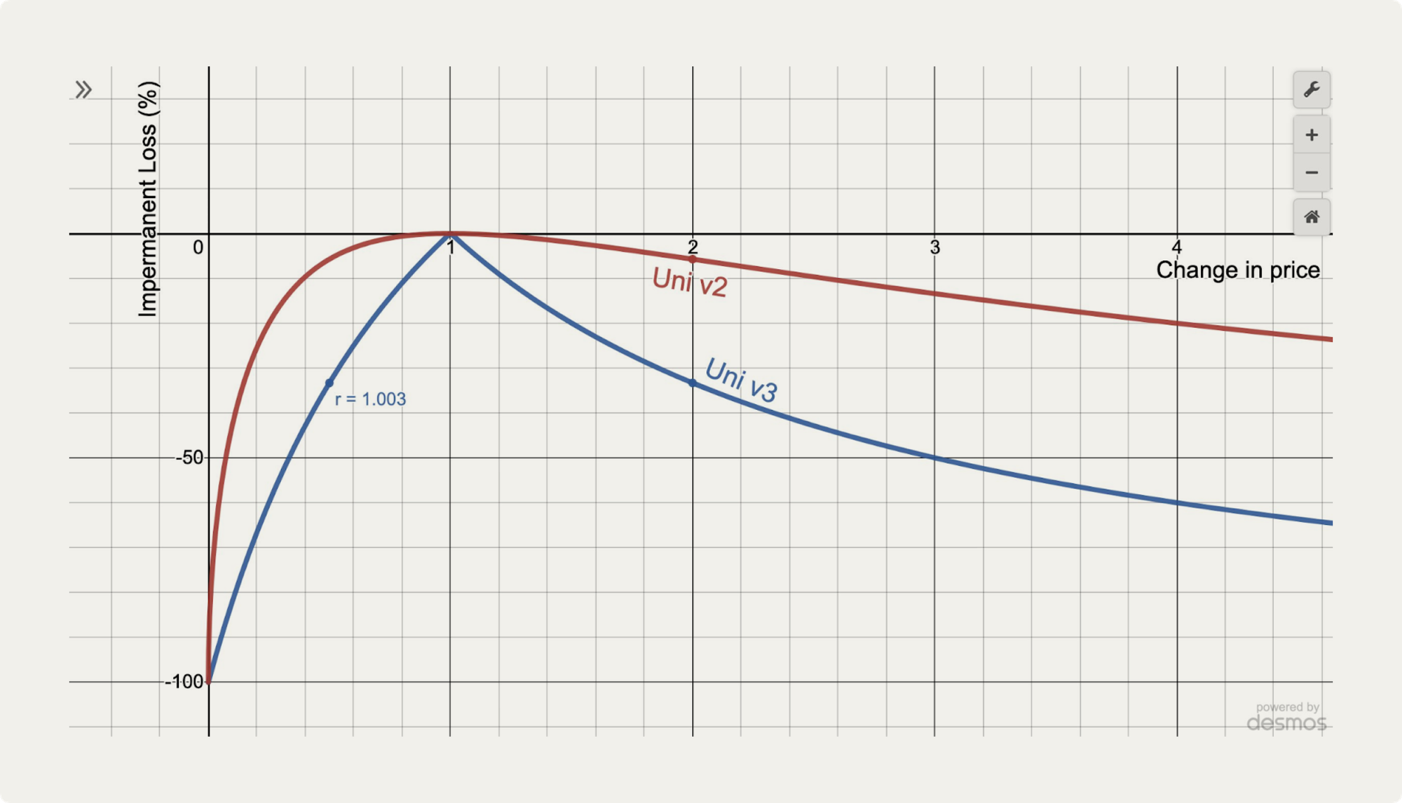
The Impermanent Loss Challenge

Traditional LP positions suffer from impermanent loss—a systematic drag on returns when asset prices move in any direction. For a pair with 20% price movement, LPs experience roughly 1% impermanent loss. With crypto's extreme volatility, this can significantly erode returns. Here’s a visualisation:

Innovations in LP Strategies

Recent innovations have improved the LP landscape:

Concentrated Liquidity (Uniswap V3): By focusing liquidity in specific price ranges, LPs can potentially increase capital efficiency, though with increased complexity and active management requirements.

Delta-Neutral Strategies: These aim to hedge impermanent loss through offsetting positions, though they typically introduce counterparty risk and increased gas costs.

While these innovations show promise, they introduce significant operational complexity and often require active management, contradicting our commitment to systematic, transparent approaches accessible to all users.

The Future of LP Integration

As these strategies mature and become more systematically implementable, Levva may selectively integrate them into specific portfolio strategies, particularly for the "Brave" category. This would require:

1. Development of robust IL-mitigation algorithms
2. Automated range management for concentrated liquidity
3. Gas-efficient rebalancing mechanisms
4. Comprehensive backtest verification across market regimes

Until then, we maintain our focus on lending and yield-bearing tokens as the core of our "Safe Yield" allocation.

A Balanced View on Token Rewards

Similarly, we take a nuanced view on token incentives and "yield farming":

Challenges with Token Rewards:

• Typically follow a predictable decay curve
• Often experience significant selling pressure
• Require constant monitoring and repositioning
• Entails substantial gas costs for smaller portfolios

Potential for Systematic Approaches:

• Rules-based harvesting and conversion to stablecoins
• Diversification across multiple reward programs
• Risk-adjusted weighting based on token fundamentals
• Automated compounding mechanisms

Rather than dismissing token rewards entirely, Levva is developing systematic approaches to selectively capture these opportunities, particularly for the "Brave" portfolio category, while maintaining rigorous risk management.

Mapping Users to Risk Profiles: Beyond Simple Categorization

One of the most challenging aspects of portfolio management is accurately assessing risk tolerance. At Levva, we approach this through a multidimensional assessment:

1. Objective Financial Circumstances

• Investment time horizon
• Liquidity needs
• Portfolio size relative to total wealth
• Age and life stage

2. Subjective Risk Tolerance

• Behavioral questionnaire responses
• Maximum drawdown tolerance
• Investment goals (preservation vs. growth)
• Prior investment experience

3. Revealed Preferences

• Past investment behavior
• Reaction to market volatility
• Portfolio adjustment frequency

This comprehensive assessment helps match users with the appropriate portfolio strategy:

Behavioral Safeguards

Recognizing that emotional biases can lead users to deviate from their optimal strategy, we at Levva consider implementing the following behavioral safeguards:

Cooling-Off Periods: Major allocation changes require a 24-hour confirmation period, reducing impulsive decisions during market volatility.

Visual Decision Aids: When users attempt to modify allocations, they see visualizations of how similar changes would have performed historically, highlighting the benefits of sticking to systematic approaches.

Scenario Testing: Users can simulate portfolio performance under various market conditions, helping them understand potential downsides before market stress occurs.

Automated Rebalancing: By default, portfolios automatically rebalance to target allocations, reducing the temptation to time markets or chase performance.

These safeguards help bridge the gap between theoretical portfolio optimization and real-world investor behavior.

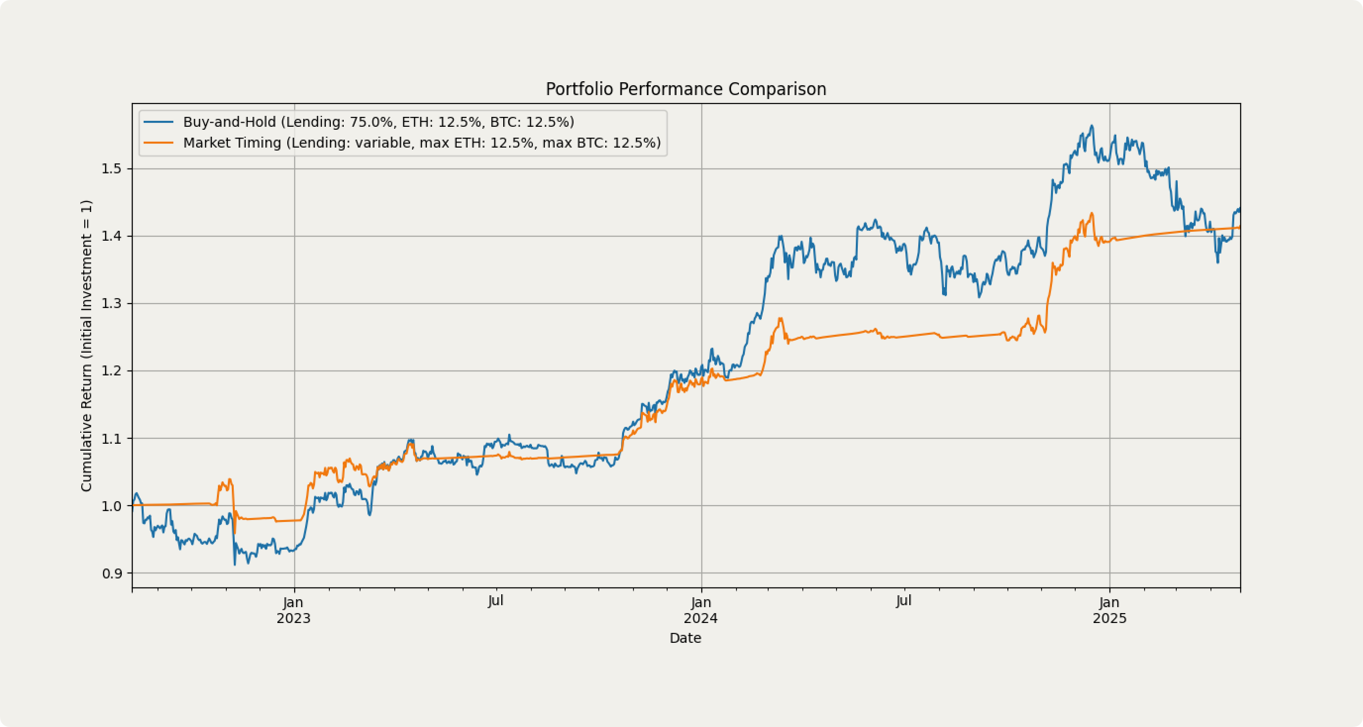
Enhancing Returns: Market Timing

The correlation variability we've observed across different market regimes provides additional rationale for incorporating tactical adjustments to our strategic allocations. While our core approach remains systematic asset allocation, we incorporate sophisticated enhancements to improve risk-adjusted returns:

Medium-Term Momentum Signals

Our research shows that 30-60 day momentum signals can improve the timing of volatile asset allocation. During negative momentum periods, we systematically reduce volatile asset exposure through various techniques.

This approach is particularly valuable given what we now understand about correlation behavior:

• During uptrends (when momentum is positive), correlations tend to be higher (0.75-0.85 range)
• During accumulation phases (often with mixed momentum signals), correlations are typically lower and more variable (0.40-0.75 range)
• Using momentum as an overlay allows us to maintain our simplified asset model while still adapting to these changing market dynamics

The chart below shows the performance improvement from adding momentum-based adjustments to our Maximum GM portfolio: curious minds can play around with this Python notebook.

Adapting to DeFi Innovation

DeFi evolves rapidly, with new yield sources, protocols, and strategies emerging regularly. How does Levva's systematic approach adapt to this innovation?

We employ a structured framework for evaluating new opportunities:

1. Risk-Adjusted Return Assessment: Analyzing expected returns against identifiable risks
2. Protocol Diligence: Audits, team background, governance structure, community support
3. Track Record: Minimum operational history requirements based on complexity
4. Operational Complexity: Gas costs, monitoring requirements, integration difficulty
5. Sustainability Analysis: Token economics, incentive alignment, long-term viability

New strategies may be first implemented in limited capacity, with exposure caps gradually increasing as they demonstrate reliability. This allows us to incorporate innovation while maintaining our commitment to systematic risk management.

Practical Implementation: The Levva Difference

Translating portfolio theory into practical implementation requires sophisticated systems and safeguards:

1. Automated Execution: Programmatic implementation of allocation strategies
2. Dynamic Rebalancing: Threshold-based rebalancing when weights deviate by ±2.5%
3. Concentration Limits: Caps on individual protocol exposure (e.g., 50% for Aave, 20% for Levva)
4. Slippage Protection: Maximum 0.1% combined slippage for entry/exit transactions
5. Circuit Breakers: Automatic trading suspension during extreme market volatility
6. Oracle Redundancy: Multiple price verification sources for trade execution

These operational safeguards ensure that theoretical portfolio optimization translates into practical benefits for vault users.

Systematic vs. Discretionary: The Evidence

The debate between systematic and discretionary approaches isn't unique to DeFi—it spans decades of traditional finance research. The evidence consistently favors systematic approaches:

1. Statistical Reality: In TradFi, 80-90% of active managers underperform market indices over 10+ year periods
2. Selection Challenge: Identifying winning tokens before they outperform is statistically unlikely
3. Survivorship Bias: The few successful token picks overshadow the many failed ones
4. Psychological Factors: Emotional biases systematically harm discretionary performance

Our analysis of crypto markets shows similar patterns. When we analyzed the performance of the top 30 non-stablecoin tokens by market cap from 2021, we found:

• Only 23% outperformed a systematic 75/25 Safe/Volatile portfolio on a risk-adjusted basis
• 60% underperformed even the most conservative Maximum SR portfolio
• The median Sharpe ratio was 0.21 vs. 0.44 for our Maximum GM portfolio

Conclusion: The Science of DeFi Portfolio Construction

The evidence is clear: for most DeFi investors, systematic portfolio construction delivers superior risk-adjusted returns compared to discretionary token selection. By understanding your risk tolerance and investment horizon, you can select the appropriate portfolio strategy:

• Ultra Safe (Maximum SR): Optimizes risk-adjusted returns with minimal volatility
• Safe (Risk Parity): Balances risk contribution for modest exposure to volatile assets
• Brave (Maximum GM): Maximizes long-term growth with controlled volatility exposure

Importantly, all these approaches maintain significant allocation to "Safe Yield" components—even our most aggressive portfolio keeps 72.5% in lower-volatility assets. This isn't conservative; it's mathematically optimal based on the geometric compounding principles discussed in our previous article.

Your Next Steps

Ready to implement these insights in your own DeFi strategy?

1. Take Our Risk Assessment: Discover which portfolio strategy aligns with your goals and risk tolerance
2. Explore Levva's Vaults: See our systematic strategies in action with real-time performance data
3. Join Our Community: Connect with like-minded investors focused on systematic DeFi strategies
4. Stay Informed: Subscribe to our updates on portfolio performance and new strategy developments

In a space dominated by speculation and narrative-chasing, systematic portfolio construction may seem boring. But as Warren Buffett famously observed, "Investing should be more like watching paint dry or watching grass grow. If you want excitement, take $800 and go to Las Vegas."

In our next article, we'll explore risk management in action, examining how rebalancing mechanisms, concentration limits, and execution safeguards protect portfolio performance during market stress.